Generative Adversarial Networks (GANs) are one of the hot topics within Deep Learning right now and are applied to various tasks, ranging from un/semi-supervised learning to generating images. These networks were originally introduced by Ian Goodfellow et al. in 2014:

We propose a new framework for estimating generative models via an adversarial process, in which we simultaneously train two models: a generative model G that captures the data distribution, and a discriminative model D that estimates the probability that a sample came from the training data rather than G. The training procedure for G is to maximize the probability of D making a mistake. This framework corresponds to a minimax two-player game. (arXiv source)

In this post I’ll show you my first experiments with these types of networks. As with almost any new technique we will apply it to a common benchmark dataset, in this case MNIST. MNIST is particular useful as its images are only small (28x28 pixels) and have only 1 color; this makes generating images a lot more feasible. After reading this post you should be able to generate your own fake handcomputerwritten digits!

Just to note: GANs are very hard to train and require a lot of tuning to get working. I tried many different setups and parameters before I got the results of this post. Even something small as changing the optimizer or tuning the learning rate can have large effects. So, if you are starting with GANs, prepare yourself for a lot of tweaking!

For convenience I use Keras (and Python 3.5) in this tutorial as it is less verbose than, for example, Tensorflow. Though, these results can easily be reproduced using other frameworks. The networks were trained using a Tensorflow backend on a Titan X GPU. These examples can also be trained on smaller GPUs, just change the batch size accordingly.

The full source code of this post is also available as a Jupyter notebook and can be found in my deep learning resource repository.

Let’s dive in!

Defining the discriminator

In our two-player game the discriminator takes the role of the police: given an image it has to determine whether the image is fake or not. With this requirement, the input of our discriminator network is a (28x28x1) input patch, equal to the dimensions of a single MNIST image. The output is a single node (1 for real, 0 for fake). The setup of the networks is roughly based on the DCGAN paper and one of its implementations.

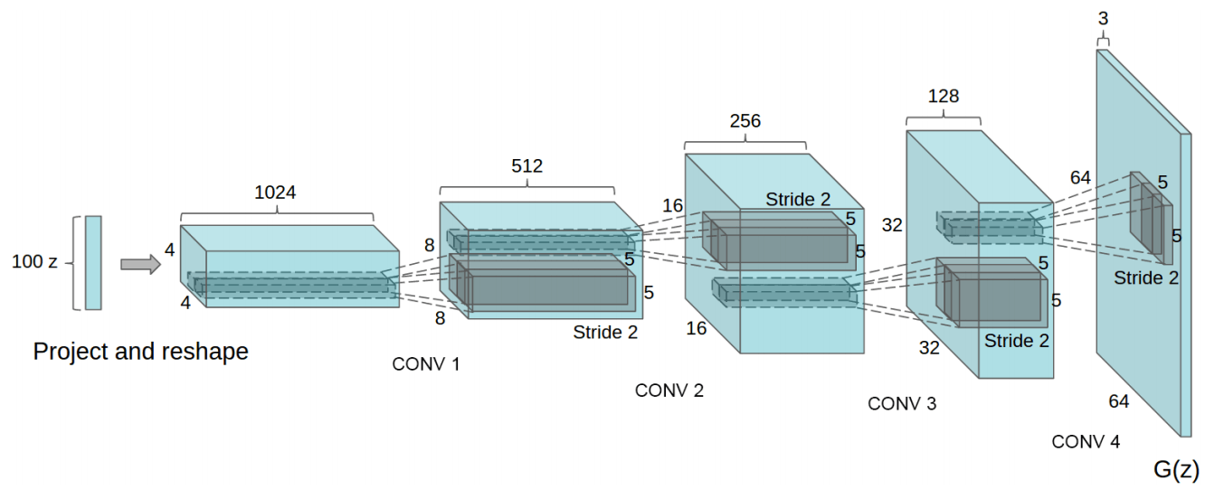
The network definition is defined below using a Keras Sequential model. I use LeakyReLU in between the convolution layers to improve the gradients.

def discriminator():
    
    net = Sequential()
    input_shape = (28, 28, 1)
    dropout_prob = 0.4

    net.add(Conv2D(64, 5, strides=2, input_shape=input_shape, padding='same'))
    net.add(LeakyReLU())
    
    net.add(Conv2D(128, 5, strides=2, padding='same'))
    net.add(LeakyReLU())
    net.add(Dropout(dropout_prob))
    
    net.add(Conv2D(256, 5, strides=2, padding='same'))
    net.add(LeakyReLU())
    net.add(Dropout(dropout_prob))
    
    net.add(Conv2D(512, 5, strides=1, padding='same'))
    net.add(LeakyReLU())
    net.add(Dropout(dropout_prob))
    
    net.add(Flatten())
    net.add(Dense(1))
    net.add(Activation('sigmoid'))
    
    return net

The full network structure is as follows:

Layer (type) Output Shape Param #

conv2d_1 (Conv2D) (None, 14, 14, 64) 1664

leaky_re_lu_1 (LeakyReLU) (None, 14, 14, 64) 0

conv2d_2 (Conv2D) (None, 7, 7, 128) 204928

leaky_re_lu_2 (LeakyReLU) (None, 7, 7, 128) 0

dropout_1 (Dropout) (None, 7, 7, 128) 0

conv2d_3 (Conv2D) (None, 4, 4, 256) 819456

leaky_re_lu_3 (LeakyReLU) (None, 4, 4, 256) 0

dropout_2 (Dropout) (None, 4, 4, 256) 0

conv2d_4 (Conv2D) (None, 4, 4, 512) 3277312

leaky_re_lu_4 (LeakyReLU) (None, 4, 4, 512) 0

dropout_3 (Dropout) (None, 4, 4, 512) 0

flatten_1 (Flatten) (None, 8192) 0

dense_1 (Dense) (None, 1) 8193

activation_1 (Activation) (None, 1) 0

Total params: 4,311,553 Trainable params: 4,311,553 Non-trainable params: 0

Defining the generator

The task of the generator, also known as “the counterfeiter”, is to fool the discriminator by producing real-looking images. These images should eventually resemble the data distribution of the MNIST dataset. The generator uses random noise as input.

The structure of the generator is comparable to the discriminator but in reverse. We start with a random vector of noise (length=100) and gradually upsample. To improve the output of the generator we use UpSampling2D and normal convolutions instead of transposed convolutions (see also this article). The sizes of the layers are adjusted to match the size of our data (28x28 as opposed to the 64x64 of the DCGAN paper). Batch normalization is added to improve stability.

def generator():
    
    net = Sequential()
    dropout_prob = 0.4
    
    net.add(Dense(7*7*256, input_dim=100))
    net.add(BatchNormalization(momentum=0.9))
    net.add(LeakyReLU())
    net.add(Reshape((7,7,256)))
    net.add(Dropout(dropout_prob))
    
    net.add(UpSampling2D())
    net.add(Conv2D(128, 5, padding='same'))
    net.add(BatchNormalization(momentum=0.9))
    net.add(LeakyReLU())
    
    net.add(UpSampling2D())
    net.add(Conv2D(64, 5, padding='same'))
    net.add(BatchNormalization(momentum=0.9))
    net.add(LeakyReLU())
    
    net.add(Conv2D(32, 5, padding='same'))
    net.add(BatchNormalization(momentum=0.9))
    net.add(LeakyReLU())
    
    net.add(Conv2D(1, 5, padding='same'))
    net.add(Activation('sigmoid'))
    
    return net

The full network of the generator looks as follows:

Layer (type) Output Shape Param #

dense_2 (Dense) (None, 12544) 1266944

batch_normalization_1 (Batch (None, 12544) 50176

leaky_re_lu_5 (LeakyReLU) (None, 12544) 0

reshape_1 (Reshape) (None, 7, 7, 256) 0

dropout_4 (Dropout) (None, 7, 7, 256) 0

up_sampling2d_1 (UpSampling2 (None, 14, 14, 256) 0

conv2d_5 (Conv2D) (None, 14, 14, 128) 819328

batch_normalization_2 (Batch (None, 14, 14, 128) 512

leaky_re_lu_6 (LeakyReLU) (None, 14, 14, 128) 0

up_sampling2d_2 (UpSampling2 (None, 28, 28, 128) 0

conv2d_6 (Conv2D) (None, 28, 28, 64) 204864

batch_normalization_3 (Batch (None, 28, 28, 64) 256

leaky_re_lu_7 (LeakyReLU) (None, 28, 28, 64) 0

conv2d_7 (Conv2D) (None, 28, 28, 32) 51232

batch_normalization_4 (Batch (None, 28, 28, 32) 128

leaky_re_lu_8 (LeakyReLU) (None, 28, 28, 32) 0

conv2d_8 (Conv2D) (None, 28, 28, 1) 801

activation_2 (Activation) (None, 28, 28, 1) 0

Total params: 2,394,241 Trainable params: 2,368,705 Non-trainable params: 25,536

Creating the models

We now defined the two separate networks but these still need to be combined into trainable models: one to train the discriminator and one to train the generator. We first start with the most simple one which is the discriminator model.

For the discriminator model we only have to define the optimizer, all the other parts of the model are already defined. I have tested both SGD, RMSprop and Adam for the optimizer of the discriminator but RMSprop performed best. RMSprop is used a low learning rate and I clip the values between -1 and 1. A small decay in the learning rate can help with stabilizing. Besides the loss we also tell Keras to gives us the accuracy as a metric.

optim_discriminator = RMSprop(lr=0.0008, clipvalue=1.0, decay=1e-10)
model_discriminator = Sequential()
model_discriminator.add(net_discriminator)
model_discriminator.compile(loss='binary_crossentropy', optimizer=optim_discriminator, metrics=['accuracy'])

================================================================= Total params: 4,311,553 Trainable params: 4,311,553 Non-trainable params: 0

It is important to note that we add the discriminator network to a new Sequential model and do not directly compile the discriminator itself. We do this because the discriminator is also required in the next step and we are able to do so by adding it to a new model before compiling.

Freezing a model

The model for the generator is a bit more complex. The generator needs to fool the discriminator by generating images. So, to train the generator we need to assess its performance on the output of the discriminator. For this we add both networks to a combined model: the adversarial model. Our adversarial model uses random noise as its input, and outputs the eventual prediction of the discriminator on the generated images. This why we added the discriminator to a new model in the previous step, by doing so we are able to reuse the network here.

The generator performs well if the adversarial model outputs ‘real’ on all inputs. In other words, for any random noise vector of the adversarial network, we aim to get an output classifying the generated image as real. Consequently this means that the discriminator failed (which is a good thing for the generator). This is the core idea of the two-player game. As input for the adversarial model we have a list of noise vectors, as target vector for the model we have a list of ones.

If we would use normal back propagation here on the full adversarial model we would slowly push the discriminator to update itself and start classifying fake images as real. Namely, the target vector of the adversarial model consists of all ones. To prevent this we must freeze the part of the model that belongs to the discriminator.

In Keras freezing a model is easily done by freezing all the layers of the model. By setting the trainable parameter to False we prevent the layer of updating within this particular model, while still being trainable in the discriminator model.

The adversarial model uses Adam as the optimizer with the default values for the momentum.

optim_adversarial = Adam(lr=0.0004, clipvalue=1.0, decay=1e-10)
model_adversarial = Sequential()
model_adversarial.add(net_generator)

# Disable layers in discriminator
for layer in net_discriminator.layers:
    layer.trainable = False

model_adversarial.add(net_discriminator)
model_adversarial.compile(loss='binary_crossentropy', optimizer=optim_adversarial, metrics=['accuracy'])

================================================================= Total params: 6,705,794 Trainable params: 2,368,705 Non-trainable params: 4,337,089

Note that the number of non-trainable parameters is very high as it excludes all parameters of the discriminator. This is exactly what we want!

Reading MNIST data

We can now load our training data. For this I use a small utility function from Tensorflow.

# Read MNIST data
x_train = input_data.read_data_sets("mnist", one_hot=True).train.images
x_train = x_train.reshape(-1, 28, 28, 1).astype(np.float32)

Training the GAN

With our models defined and the data loaded we can start training our GAN. The models are trained one after another, starting with the discriminator. The discriminator is trained on a set of both fake and real images and tries to classify them correctly. The adversarial model is trained on noise vectors as explained above.

This setup (where the models alternate) is the most easy setup. For more complex images other strategies can be used. You can, for example, let the generator train more often than the discriminator to force it to become better.

batch_size = 256

for i in range(3001):
    
    # Select a random set of training images from the mnist dataset
    images_train = x_train[np.random.randint(0, x_train.shape[0], size=batch_size), :, :, :]
    # Generate a random noise vector
    noise = np.random.uniform(-1.0, 1.0, size=[batch_size, 100])
    # Use the generator to create fake images from the noise vector
    images_fake = net_generator.predict(noise)
    
    # Create a dataset with fake and real images
    x = np.concatenate((images_train, images_fake))
    y = np.ones([2*batch_size, 1])
    y[batch_size:, :] = 0 

    # Train discriminator for one batch
    d_stats = model_discriminator.train_on_batch(x, y)
    
    # Train the generator
    # The input of th adversarial model is a list of noise vectors. The generator is 'good' if the discriminator classifies
    # all the generated images as real. Therefore, the desired output is a list of all ones.
    y = np.ones([batch_size, 1])
    noise = np.random.uniform(-1.0, 1.0, size=[batch_size, 100])
    a_stats = model_adversarial.train_on_batch(noise, y)

Note: All the plotting functionality was removed from the above snippet. See the GitHub repository for the full code.

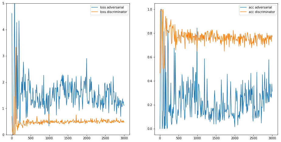
Result of training

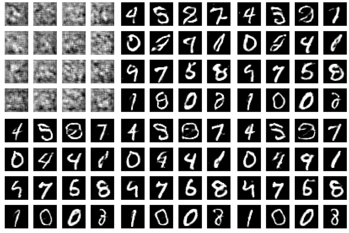
After 3000 iterations we have a generator that is able to generate images that most of the time resemble MNIST digits. When we train longer, I stopped at 10.000, the network performs even better. Not all generated images are great but this could be resolved with more tuning and training.

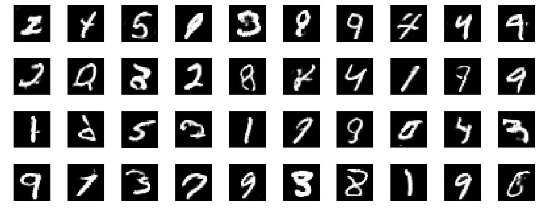
Exploring the noise vector

Now that we have a working generator we can further explore the generation process. Some examples are shown below.

Morphing instances

By tuning the noise vector we can get some insights in how the generator works. Primarily how the noise vector maps to the generated digits. For example, if we slowly change a noise vector filled with zeros to one filled with ones we see a digit 3 slowly changing in to a 4.

plt.figure(figsize=(15,4))

for i in range(10):
    noise = np.zeros([1,100]) - 1 + (i * 0.2)
    images = net_generator.predict(noise)
    
    image = images[0, :, :, :]
    image = np.reshape(image, [28, 28])
          
    plt.subplot(1, 10, i+1)
    plt.imshow(image, cmap='gray')
    plt.axis('off')

plt.tight_layout()
plt.show()
    
    

Combining noise vectors

As the noise vectors are just numbers we can also do some math with it. With digits this is not that spectacular, but when you imagine that you can also do this with generated images of real objects the possibilities become very interesting. E.g. combining the noise vector of a man with the noise vector of a woman wearing glasses and afterwards remove the encoding for ‘woman’.

In this example we show simple addition. The noise vector for a 3 combined with one for a 8 morphs in to something that resembles a 4.

a = np.random.uniform(-1.0, 1.0, size=[1, 100])
b = np.random.uniform(-1.0, 1.0, size=[1, 100])

image_a = np.reshape(net_generator.predict(a)[0], [28, 28])
image_b = np.reshape(net_generator.predict(b)[0], [28, 28])
image_sum = np.reshape(net_generator.predict(b - a)[0], [28, 28])

plt.figure(figsize=(5,4))

plt.subplot(1,3,1)
plt.imshow(image_a, cmap='gray')
plt.axis('off')

plt.subplot(1,3,2)
plt.imshow(image_b, cmap='gray')
plt.axis('off')

plt.subplot(1,3,3)
plt.imshow(image_sum, cmap='gray')
plt.axis('off')

plt.tight_layout()
plt.show()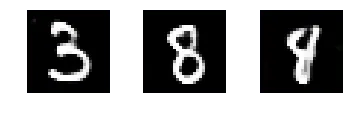

Final results

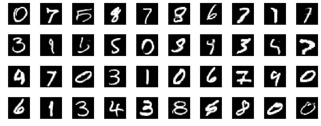
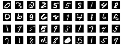
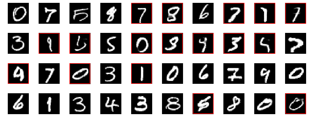
Remember the image with digits at the start? Did you see which ones were fake and which ones were real? The fake ones are outlined in the image below.

I hope you liked this post and found it useful. Do you have any feedback, ideas or other comments? Please leave them at the comments below!

Next step

Want to learn more about GANs? Please see part 2 of this series where I apply GANs to RGB images: “Getting started with GANs (Part 2): Colorful MNIST”.